How To Draw T Distribution Curve

Diagnostic plot

Terminology and derivations
from a confusion matrix

condition positive (P) the number of existent positive cases in the information condition negative (N) the number of existent negative cases in the data true positive (TP) A test result that correctly indicates the presence of a condition or characteristic true negative (TN) A test result that correctly indicates the absence of a condition or characteristic false positive (FP) A exam event which wrongly indicates that a particular status or attribute is present false negative (FN) A test result which wrongly indicates that a item status or attribute is absent-minded sensitivity, recall, hit rate, or truthful positive rate (TPR) ${\displaystyle \mathrm {TPR} ={\frac {\mathrm {TP} }{\mathrm {P} }}={\frac {\mathrm {TP} }{\mathrm {TP} +\mathrm {FN} }}=1-\mathrm {FNR} }$ specificity, selectivity or true negative rate (TNR) ${\displaystyle \mathrm {TNR} ={\frac {\mathrm {TN} }{\mathrm {Due north} }}={\frac {\mathrm {TN} }{\mathrm {TN} +\mathrm {FP} }}=1-\mathrm {FPR} }$ precision or positive predictive value (PPV) ${\displaystyle \mathrm {PPV} ={\frac {\mathrm {TP} }{\mathrm {TP} +\mathrm {FP} }}=i-\mathrm {FDR} }$ negative predictive value (NPV) ${\displaystyle \mathrm {NPV} ={\frac {\mathrm {TN} }{\mathrm {TN} +\mathrm {FN} }}=1-\mathrm {FOR} }$ miss rate or false negative rate (FNR) ${\displaystyle \mathrm {FNR} ={\frac {\mathrm {FN} }{\mathrm {P} }}={\frac {\mathrm {FN} }{\mathrm {FN} +\mathrm {TP} }}=1-\mathrm {TPR} }$ fall-out or false positive rate (FPR) ${\displaystyle \mathrm {FPR} ={\frac {\mathrm {FP} }{\mathrm {North} }}={\frac {\mathrm {FP} }{\mathrm {FP} +\mathrm {TN} }}=1-\mathrm {TNR} }$ false discovery rate (FDR) ${\displaystyle \mathrm {FDR} ={\frac {\mathrm {FP} }{\mathrm {FP} +\mathrm {TP} }}=1-\mathrm {PPV} }$ false omission rate (FOR) ${\displaystyle \mathrm {FOR} ={\frac {\mathrm {FN} }{\mathrm {FN} +\mathrm {TN} }}=one-\mathrm {NPV} }$ Positive likelihood ratio (LR+) ${\displaystyle \mathrm {LR+} ={\frac {\mathrm {TPR} }{\mathrm {FPR} }}}$ Negative likelihood ratio (LR-) ${\displaystyle \mathrm {LR-} ={\frac {\mathrm {FNR} }{\mathrm {TNR} }}}$ prevalence threshold (PT) ${\displaystyle \mathrm {PT} ={\frac {{\sqrt {\mathrm {TPR} (-\mathrm {TNR} +1)}}+\mathrm {TNR} -1}{(\mathrm {TPR} +\mathrm {TNR} -1)}}={\frac {\sqrt {\mathrm {FPR} }}{{\sqrt {\mathrm {TPR} }}+{\sqrt {\mathrm {FPR} }}}}}$ threat score (TS) or critical success index (CSI) ${\displaystyle \mathrm {TS} ={\frac {\mathrm {TP} }{\mathrm {TP} +\mathrm {FN} +\mathrm {FP} }}}$ Prevalence ${\displaystyle {\frac {\mathrm {P} }{\mathrm {P} +\mathrm {North} }}}$ accuracy (ACC) ${\displaystyle \mathrm {ACC} ={\frac {\mathrm {TP} +\mathrm {TN} }{\mathrm {P} +\mathrm {Due north} }}={\frac {\mathrm {TP} +\mathrm {TN} }{\mathrm {TP} +\mathrm {TN} +\mathrm {FP} +\mathrm {FN} }}}$ counterbalanced accuracy (BA) ${\displaystyle \mathrm {BA} ={\frac {TPR+TNR}{2}}}$ F1 score is the harmonic mean of precision and sensitivity: ${\displaystyle \mathrm {F} _{ane}=2\times {\frac {\mathrm {PPV} \times \mathrm {TPR} }{\mathrm {PPV} +\mathrm {TPR} }}={\frac {2\mathrm {TP} }{2\mathrm {TP} +\mathrm {FP} +\mathrm {FN} }}}$ phi coefficient (φ or rφ) or Matthews correlation coefficient (MCC) ${\displaystyle \mathrm {MCC} ={\frac {\mathrm {TP} \times \mathrm {TN} -\mathrm {FP} \times \mathrm {FN} }{\sqrt {(\mathrm {TP} +\mathrm {FP} )(\mathrm {TP} +\mathrm {FN} )(\mathrm {TN} +\mathrm {FP} )(\mathrm {TN} +\mathrm {FN} )}}}}$ Fowlkes–Mallows index (FM) ${\displaystyle \mathrm {FM} ={\sqrt {{\frac {TP}{TP+FP}}\times {\frac {TP}{TP+FN}}}}={\sqrt {PPV\times TPR}}}$ informedness or bookmaker informedness (BM) ${\displaystyle \mathrm {BM} =\mathrm {TPR} +\mathrm {TNR} -1}$ markedness (MK) or deltaP (Δp) ${\displaystyle \mathrm {MK} =\mathrm {PPV} +\mathrm {NPV} -1}$ Diagnostic odds ratio (DOR) ${\displaystyle \mathrm {DOR} ={\frac {\mathrm {LR+} }{\mathrm {LR-} }}}$ Sources: Fawcett (2006),[1] Piryonesi and El-Diraby (2020),[2] Powers (2011),[3] Ting (2011),[4] CAWCR,[5] D. Chicco & G. Jurman (2020, 2021),[6] [7] Tharwat (2018).[8]

ROC curve of three predictors of peptide cleaving in the proteasome.

A receiver operating characteristic curve, or ROC curve, is a graphical plot that illustrates the diagnostic ability of a binary classifier system every bit its discrimination threshold is varied. The method was originally developed for operators of military radar receivers starting in 1941, which led to its name.

The ROC curve is created by plotting the true positive rate (TPR) confronting the false positive charge per unit (FPR) at various threshold settings. The true-positive charge per unit is too known as sensitivity, recollect or probability of detection.^[9] The false-positive charge per unit is too known as probability of faux alarm ^[9] and can be calculated equally (1 − specificity). Information technology tin also exist thought of as a plot of the power as a role of the Blazon I Mistake of the conclusion rule (when the operation is calculated from merely a sample of the population, it tin can be thought of as estimators of these quantities). The ROC curve is thus the sensitivity or recall as a part of autumn-out. In general, if the probability distributions for both detection and false alert are known, the ROC curve tin can exist generated by plotting the cumulative distribution office (area under the probability distribution from ${\displaystyle -\infty }$ to the discrimination threshold) of the detection probability in the y-axis versus the cumulative distribution role of the false-alert probability on the x-axis.

ROC analysis provides tools to select possibly optimal models and to discard suboptimal ones independently from (and prior to specifying) the cost context or the class distribution. ROC analysis is related in a direct and natural way to cost/benefit assay of diagnostic decision making.

The ROC curve was first developed past electrical engineers and radar engineers during World War II for detecting enemy objects in battlefields and was presently introduced to psychology to account for perceptual detection of stimuli. ROC assay since then has been used in medicine, radiology, biometrics, forecasting of natural hazards,^[10] meteorology,^[11] model performance assessment,^[12] and other areas for many decades and is increasingly used in motorcar learning and information mining research.

The ROC is besides known equally a relative operating characteristic curve, because information technology is a comparison of two operating characteristics (TPR and FPR) equally the criterion changes.^[xiii]

Basic concept [edit]

A classification model (classifier or diagnosis^[14]) is a mapping of instances between certain classes/groups. Considering the classifier or diagnosis result can be an arbitrary real value (continuous output), the classifier purlieus betwixt classes must be determined past a threshold value (for instance, to decide whether a person has hypertension based on a blood pressure measure). Or it tin can be a discrete class label, indicating one of the classes.

Consider a two-class prediction trouble (binary classification), in which the outcomes are labeled either equally positive (p) or negative (n). There are 4 possible outcomes from a binary classifier. If the outcome from a prediction is p and the bodily value is also p, then it is called a true positive (TP); however if the actual value is n and so it is said to exist a false positive (FP). Conversely, a true negative (TN) has occurred when both the prediction result and the bodily value are n, and false negative (FN) is when the prediction outcome is n while the actual value is p.

To get an appropriate example in a real-world problem, consider a diagnostic test that seeks to determine whether a person has a certain disease. A false positive in this example occurs when the person tests positive, but does not really have the disease. A imitation negative, on the other paw, occurs when the person tests negative, suggesting they are healthy, when they actually practice have the disease.

Let u.s. define an experiment from P positive instances and N negative instances for some condition. The four outcomes can be formulated in a 2×2 contingency tabular array or defoliation matrix, as follows:

		Predicted condition		Sources: [15] [xvi] [17] [18] [19] [20] [21] [22] view talk edit
	Total population = P + North	Positive (PP)	Negative (PN)	Informedness, bookmaker informedness (BM) = TPR + TNR − i	Prevalence threshold (PT) = √TPR × FPR − FPR / TPR − FPR
Actual condition	Positive (P)	True positive (TP), striking	False negative (FN), type 2 error, miss, underestimation	True positive rate (TPR), recall, sensitivity (SEN), probability of detection, hit rate, ability = TP / P = i − FNR	False negative rate (FNR), miss charge per unit = FN / P = 1 − TPR
	Negative (N)	False positive (FP), type I error, false alarm, overestimation	Truthful negative (TN), correct rejection	Imitation positive rate (FPR), probability of false alarm, fall-out = FP / N = 1 − TNR	True negative rate (TNR), specificity (SPC), selectivity = TN / Northward = one − FPR
	Prevalence = P / P + N	Positive predictive value (PPV), precision = TP / PP = one − FDR	False omission rate (FOR) = FN / PN = 1 − NPV	Positive likelihood ratio (LR+) = TPR / FPR	Negative likelihood ratio (LR−) = FNR / TNR
	Accuracy (ACC) = TP + TN / P + Due north	False discovery rate (FDR) = FP / PP = i − PPV	Negative predictive value (NPV) = TN / PN = one − FOR	Markedness (MK), deltaP (Δp) = PPV + NPV − one	Diagnostic odds ratio (DOR) = LR+ / LR−
	Balanced accuracy (BA) = TPR + TNR / 2	Fi score = 2 PPV × TPR / PPV + TPR = 2 TP / 2 TP + FP + FN	Fowlkes–Mallows index (FM) = √PPV×TPR	Matthews correlation coefficient (MCC) = √TPR×TNR×PPV×NPV − √FNR×FPR×FOR×FDR	Threat score (TS), disquisitional success index (CSI), Jaccard index = TP / TP + FN + FP

ROC infinite [edit]

The ROC space and plots of the 4 prediction examples.

The ROC space for a "better" and "worse" classifier.

The contingency table can derive several evaluation "metrics" (run into infobox). To describe a ROC bend, only the true positive rate (TPR) and imitation positive charge per unit (FPR) are needed (every bit functions of some classifier parameter). The TPR defines how many correct positive results occur among all positive samples available during the test. FPR, on the other hand, defines how many incorrect positive results occur among all negative samples available during the test.

A ROC space is defined by FPR and TPR as ten and y axes, respectively, which depicts relative trade-offs between truthful positive (benefits) and false positive (costs). Since TPR is equivalent to sensitivity and FPR is equal to 1 − specificity, the ROC graph is sometimes called the sensitivity vs (1 − specificity) plot. Each prediction outcome or case of a defoliation matrix represents one point in the ROC space.

The best possible prediction method would yield a point in the upper left corner or coordinate (0,1) of the ROC space, representing 100% sensitivity (no false negatives) and 100% specificity (no false positives). The (0,1) point is also called a perfect nomenclature. A random guess would give a point forth a diagonal line (the so-called line of no-discrimination) from the bottom left to the acme right corners (regardless of the positive and negative base rates).^[23] An intuitive case of random guessing is a decision by flipping coins. Equally the size of the sample increases, a random classifier's ROC point tends towards the diagonal line. In the case of a counterbalanced money, it will tend to the point (0.v, 0.5).

The diagonal divides the ROC space. Points in a higher place the diagonal represent good classification results (better than random); points below the line correspond bad results (worse than random). Annotation that the output of a consistently bad predictor could simply be inverted to obtain a good predictor.

Let u.s.a. look into four prediction results from 100 positive and 100 negative instances:

A	B	C	C′
TP=63 FN=37 100 FP=28 TN=72 100 91 109 200	TP=77 FN=23 100 FP=77 TN=23 100 154 46 200	TP=24 FN=76 100 FP=88 TN=12 100 112 88 200	TP=76 FN=24 100 FP=12 TN=88 100 88 112 200
TPR = 0.63	TPR = 0.77	TPR = 0.24	TPR = 0.76
FPR = 0.28	FPR = 0.77	FPR = 0.88	FPR = 0.12
PPV = 0.69	PPV = 0.50	PPV = 0.21	PPV = 0.86
F1 = 0.66	F1 = 0.61	F1 = 0.23	F1 = 0.81
ACC = 0.68	ACC = 0.50	ACC = 0.18	ACC = 0.82

Plots of the four results above in the ROC space are given in the figure. The effect of method A clearly shows the best predictive power among A, B, and C. The issue of B lies on the random estimate line (the diagonal line), and information technology tin can be seen in the table that the accuracy of B is l%. However, when C is mirrored beyond the heart signal (0.5,0.5), the resulting method C′ is fifty-fifty improve than A. This mirrored method but reverses the predictions of any method or exam produced the C contingency table. Although the original C method has negative predictive ability, simply reversing its decisions leads to a new predictive method C′ which has positive predictive power. When the C method predicts p or north, the C′ method would predict due north or p, respectively. In this fashion, the C′ examination would perform the best. The closer a result from a contingency table is to the upper left corner, the better it predicts, but the distance from the random guess line in either direction is the best indicator of how much predictive power a method has. If the result is below the line (i.e. the method is worse than a random gauge), all of the method'south predictions must be reversed in society to use its power, thereby moving the issue above the random guess line.

Curves in ROC space [edit]

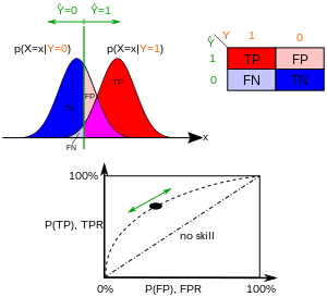
In binary classification, the course prediction for each example is oftentimes made based on a continuous random variable ${\displaystyle 10}$ , which is a "score" computed for the example (e.thou. the estimated probability in logistic regression). Given a threshold parameter ${\displaystyle T}$ , the instance is classified as "positive" if ${\displaystyle X>T}$ , and "negative" otherwise. ${\displaystyle X}$ follows a probability density ${\displaystyle f_{1}(x)}$ if the case actually belongs to form "positive", and ${\displaystyle f_{0}(x)}$ if otherwise. Therefore, the true positive rate is given by ${\displaystyle {\mbox{TPR}}(T)=\int _{T}^{\infty }f_{ane}(x)\,dx}$ and the imitation positive rate is given by ${\displaystyle {\mbox{FPR}}(T)=\int _{T}^{\infty }f_{0}(x)\,dx}$ . The ROC curve plots parametrically ${\displaystyle {\mbox{TPR}}(T)}$ versus ${\displaystyle {\mbox{FPR}}(T)}$ with ${\displaystyle T}$ as the varying parameter.

For example, imagine that the blood protein levels in diseased people and healthy people are normally distributed with ways of 2 g/dL and 1 grand/dL respectively. A medical test might measure the level of a certain protein in a blood sample and classify any number higher up a sure threshold equally indicating disease. The experimenter can adjust the threshold (green vertical line in the figure), which will in turn change the simulated positive rate. Increasing the threshold would issue in fewer false positives (and more than fake negatives), corresponding to a leftward move on the curve. The actual shape of the curve is determined past how much overlap the two distributions take.

Farther interpretations [edit]

Sometimes, the ROC is used to generate a summary statistic. Common versions are:

• the intercept of the ROC bend with the line at 45 degrees orthogonal to the no-discrimination line - the balance signal where Sensitivity = i - Specificity
• the intercept of the ROC bend with the tangent at 45 degrees parallel to the no-bigotry line that is closest to the error-complimentary signal (0,one) - also called Youden's J statistic and generalized as Informedness^{[ citation needed ]}
• the area between the ROC bend and the no-bigotry line multiplied by two is called the Gini coefficient. Information technology should non be dislocated with the measure of statistical dispersion also called Gini coefficient.
• the surface area between the full ROC curve and the triangular ROC curve including merely (0,0), (i,one) and ane selected operating betoken ${\displaystyle (tpr,fpr)}$ - Consistency^[24]
• the area nether the ROC curve, or "AUC" ("expanse under curve"), or A' (pronounced "a-prime"),^[25] or "c-statistic" ("cyclopedia statistic").^[26]
• the sensitivity index d′ (pronounced "d-prime"), the altitude between the mean of the distribution of activity in the system under noise-alone conditions and its distribution under signal-alone conditions, divided past their standard deviation, nether the assumption that both these distributions are normal with the same standard deviation. Under these assumptions, the shape of the ROC is entirely determined past d′.

However, any attempt to summarize the ROC curve into a single number loses information about the pattern of tradeoffs of the particular discriminator algorithm.

Probabilistic interpretation [edit]

When using normalized units, the area under the curve (often referred to every bit but the AUC) is equal to the probability that a classifier will rank a randomly chosen positive instance higher than a randomly called negative one (assuming 'positive' ranks higher than 'negative').^[27] In other words, when given one randomly selected positive instance and one randomly selected negative instance, AUC is the probability that the classifier will be able to tell which 1 is which.

This can be seen as follows: the expanse under the curve is given by (the integral boundaries are reversed as big threshold ${\displaystyle T}$ has a lower value on the 10-centrality)

${\displaystyle {\mbox{TPR}}(T):T\mapsto y(ten)}$

${\displaystyle {\mbox{FPR}}(T):T\mapsto x}$

${\displaystyle A=\int _{x=0}^{one}{\mbox{TPR}}({\mbox{FPR}}^{-one}(10))\,dx=\int _{\infty }^{-\infty }{\mbox{TPR}}(T){\mbox{FPR}}'(T)\,dT=\int _{-\infty }^{\infty }\int _{-\infty }^{\infty }I(T'>T)f_{ane}(T')f_{0}(T)\,dT'\,dT=P(X_{one}>X_{0})}$

where ${\displaystyle X_{1}}$ is the score for a positive case and ${\displaystyle X_{0}}$ is the score for a negative instance, and ${\displaystyle f_{0}}$ and ${\displaystyle f_{1}}$ are probability densities as defined in previous section.

Area under the bend [edit]

It tin can be shown that the AUC is closely related to the Mann–Whitney U,^{[28] [29]} which tests whether positives are ranked college than negatives. It is likewise equivalent to the Wilcoxon test of ranks.^[29] For a predictor ${\textstyle f}$ , an unbiased estimator of its AUC can exist expressed by the following Wilcoxon-Mann-Whitney statistic:^[30]

${\displaystyle AUC(f)={\frac {\sum _{t_{0}\in {\mathcal {D}}^{0}}\sum _{t_{i}\in {\mathcal {D}}^{1}}{\textbf {one}}[f(t_{0})<f(t_{1})]}{|{\mathcal {D}}^{0}|\cdot |{\mathcal {D}}^{i}|}},}$

where, ${\textstyle {\textbf {1}}[f(t_{0})<f(t_{one})]}$ denotes an indicator part which returns ane iff ${\displaystyle f(t_{0})<f(t_{1})}$ otherwise return 0; ${\displaystyle {\mathcal {D}}^{0}}$ is the set of negative examples, and ${\displaystyle {\mathcal {D}}^{i}}$ is the set of positive examples.

The AUC is related to the *Gini coefficient* ( ${\displaystyle G_{1}}$ ) by the formula ${\displaystyle G_{1}=2{\mbox{AUC}}-ane}$ , where:

${\displaystyle G_{ane}=ane-\sum _{k=one}^{n}(X_{1000}-X_{k-1})(Y_{yard}+Y_{k-1})}$ ^[31]

In this way, it is possible to calculate the AUC past using an boilerplate of a number of trapezoidal approximations. ${\displaystyle G_{1}}$ should not be confused with the measure out of statistical dispersion that is also chosen Gini coefficient.

It is also common to calculate the Area Under the ROC Convex Hull (ROC AUCH = ROCH AUC) every bit any point on the line segment between ii prediction results can be accomplished by randomly using one or the other organisation with probabilities proportional to the relative length of the opposite component of the segment.^[32] It is as well possible to capsize concavities – merely as in the figure the worse solution can be reflected to become a amend solution; concavities tin can be reflected in any line segment, but this more extreme course of fusion is much more than likely to overfit the data.^[33]

The machine learning community nearly frequently uses the ROC AUC statistic for model comparison.^[34] This practice has been questioned because AUC estimates are quite noisy and suffer from other problems.^{[35] [36] [37]} However, the coherence of AUC as a measure of aggregated classification performance has been vindicated, in terms of a uniform rate distribution,^[38] and AUC has been linked to a number of other functioning metrics such as the Brier score.^[39]

Another trouble with ROC AUC is that reducing the ROC Curve to a single number ignores the fact that information technology is about the tradeoffs between the different systems or performance points plotted and not the performance of an private system, as well as ignoring the possibility of concavity repair, so that related culling measures such every bit Informedness^{[ commendation needed ]} or DeltaP are recommended.^{[24] [40]} These measures are essentially equivalent to the Gini for a single prediction point with DeltaP' = Informedness = 2AUC-one, whilst DeltaP = Markedness represents the dual (viz. predicting the prediction from the existent grade) and their geometric mean is the Matthews correlation coefficient.^{[ citation needed ]}

Whereas ROC AUC varies between 0 and ane — with an uninformative classifier yielding 0.5 — the alternative measures known as Informedness,^{[ citation needed ]} Certainty ^[24] and Gini Coefficient (in the unmarried parameterization or single system instance)^{[ citation needed ]} all have the advantage that 0 represents chance performance whilst i represents perfect operation, and −1 represents the "perverse" case of full informedness always giving the wrong response.^[41] Bringing chance performance to 0 allows these alternative scales to be interpreted as Kappa statistics. Informedness has been shown to have desirable characteristics for Automobile Learning versus other common definitions of Kappa such every bit Cohen Kappa and Fleiss Kappa.^{[ citation needed ] [42]}

Sometimes it can exist more useful to look at a specific region of the ROC Bend rather than at the whole curve. It is possible to compute fractional AUC.^[43] For example, one could focus on the region of the curve with low false positive charge per unit, which is often of prime interest for population screening tests.^[44] Another common arroyo for classification issues in which P ≪ N (common in bioinformatics applications) is to utilize a logarithmic calibration for the x-centrality.^[45]

The ROC area nether the curve is besides called c-statistic or c statistic.^[46]

Other measures [edit]

The Total Operating Characteristic (TOC) also characterizes diagnostic power while revealing more than information than the ROC. For each threshold, ROC reveals two ratios, TP/(TP + FN) and FP/(FP + TN). In other words, ROC reveals ${\displaystyle {\frac {\text{hits}}{{\text{hits}}+{\text{misses}}}}}$ and ${\displaystyle {\frac {\text{faux alarms}}{{\text{false alarms}}+{\text{right rejections}}}}}$ . On the other hand, TOC shows the total information in the contingency table for each threshold.^[47] The TOC method reveals all of the information that the ROC method provides, plus boosted important data that ROC does not reveal, i.eastward. the size of every entry in the contingency table for each threshold. TOC besides provides the popular AUC of the ROC.^[48]

These figures are the TOC and ROC curves using the same information and thresholds. Consider the point that corresponds to a threshold of 74. The TOC curve shows the number of hits, which is 3, and hence the number of misses, which is seven. Additionally, the TOC bend shows that the number of false alarms is 4 and the number of correct rejections is xvi. At whatever given point in the ROC curve, it is possible to glean values for the ratios of ${\displaystyle {\frac {\text{false alarms}}{{\text{false alarms}}+{\text{right rejections}}}}}$ and ${\displaystyle {\frac {\text{hits}}{{\text{hits}}+{\text{misses}}}}}$ . For example, at threshold 74, it is axiomatic that the x coordinate is 0.2 and the y coordinate is 0.three. However, these ii values are bereft to construct all entries of the underlying two-past-ii contingency table.

Detection mistake tradeoff graph [edit]

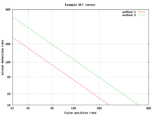
An alternative to the ROC curve is the detection error tradeoff (DET) graph, which plots the fake negative charge per unit (missed detections) vs. the simulated positive charge per unit (simulated alarms) on non-linearly transformed x- and y-axes. The transformation function is the quantile function of the normal distribution, i.e., the changed of the cumulative normal distribution. It is, in fact, the same transformation as zROC, below, except that the complement of the hit rate, the miss rate or false negative rate, is used. This alternative spends more than graph area on the region of interest. Almost of the ROC expanse is of little involvement; one primarily cares near the region tight against the y-axis and the top left corner – which, because of using miss rate instead of its complement, the hit rate, is the lower left corner in a DET plot. Furthermore, DET graphs accept the useful property of linearity and a linear threshold beliefs for normal distributions.^[49] The DET plot is used extensively in the automatic speaker recognition customs, where the name DET was get-go used. The analysis of the ROC operation in graphs with this warping of the axes was used by psychologists in perception studies halfway through the 20th century,^{[ commendation needed ]} where this was dubbed "double probability paper".^[50]

Z-score [edit]

If a standard score is applied to the ROC curve, the curve will exist transformed into a direct line.^[51] This z-score is based on a normal distribution with a mean of aught and a standard deviation of one. In memory forcefulness theory, ane must presume that the zROC is not just linear, but has a slope of ane.0. The normal distributions of targets (studied objects that the subjects need to recall) and lures (not studied objects that the subjects effort to think) is the cistron causing the zROC to be linear.

The linearity of the zROC curve depends on the standard deviations of the target and lure strength distributions. If the standard deviations are equal, the slope will be i.0. If the standard difference of the target forcefulness distribution is larger than the standard divergence of the lure strength distribution, then the slope volition be smaller than 1.0. In most studies, information technology has been found that the zROC curve slopes constantly fall below 1, usually between 0.5 and 0.9.^[52] Many experiments yielded a zROC slope of 0.viii. A slope of 0.viii implies that the variability of the target forcefulness distribution is 25% larger than the variability of the lure strength distribution.^[53]

Another variable used isd' (d prime) (discussed above in "Other measures"), which tin hands exist expressed in terms of z-values. Although d' is a commonly used parameter, it must be recognized that it is only relevant when strictly adhering to the very strong assumptions of strength theory made above.^[54]

The z-score of an ROC bend is always linear, equally assumed, except in special situations. The Yonelinas familiarity-recollection model is a two-dimensional account of recognition memory. Instead of the subject simply answering yes or no to a specific input, the subject gives the input a feeling of familiarity, which operates like the original ROC bend. What changes, though, is a parameter for Recollection (R). Recollection is causeless to be all-or-none, and it trumps familiarity. If there were no recollection component, zROC would have a predicted gradient of 1. Nevertheless, when adding the recollection component, the zROC curve will exist concave up, with a decreased slope. This difference in shape and slope result from an added element of variability due to some items being recollected. Patients with anterograde amnesia are unable to recollect, so their Yonelinas zROC curve would have a slope close to 1.0.^[55]

History [edit]

The ROC curve was first used during Earth State of war Ii for the assay of radar signals before information technology was employed in signal detection theory.^[56] Following the set on on Pearl Harbor in 1941, the United States army began new enquiry to increase the prediction of correctly detected Japanese aircraft from their radar signals. For these purposes they measured the power of a radar receiver operator to brand these important distinctions, which was called the Receiver Operating Feature.^[57]

In the 1950s, ROC curves were employed in psychophysics to assess human (and occasionally non-human beast) detection of weak signals.^[56] In medicine, ROC analysis has been extensively used in the evaluation of diagnostic tests.^{[58] [59]} ROC curves are also used extensively in epidemiology and medical research and are often mentioned in conjunction with evidence-based medicine. In radiology, ROC assay is a common technique to evaluate new radiology techniques.^[sixty] In the social sciences, ROC assay is often called the ROC Accurateness Ratio, a mutual technique for judging the accuracy of default probability models. ROC curves are widely used in laboratory medicine to assess the diagnostic accuracy of a test, to choose the optimal cut-off of a test and to compare diagnostic accuracy of several tests.

ROC curves also proved useful for the evaluation of machine learning techniques. The first application of ROC in machine learning was by Spackman who demonstrated the value of ROC curves in comparison and evaluating unlike classification algorithms.^[61]

ROC curves are besides used in verification of forecasts in meteorology.^[62]

ROC curves beyond binary classification [edit]

The extension of ROC curves for classification problems with more than two classes is cumbersome. Two common approaches for when there are multiple classes are (one) average over all pairwise AUC values^[63] and (2) compute the volume under surface (VUS).^{[64] [65]} To boilerplate over all pairwise classes, i computes the AUC for each pair of classes, using only the examples from those two classes every bit if at that place were no other classes, and then averages these AUC values over all possible pairs. When at that place are c classes there will exist c(c − 1) / 2 possible pairs of classes.

The book under surface arroyo has i plot a hypersurface rather than a curve and and then measure out the hypervolume under that hypersurface. Every possible decision rule that one might use for a classifier for c classes can exist described in terms of its true positive rates (TPR₁, ..., TPR _c ). It is this fix of rates that defines a point, and the ready of all possible decision rules yields a cloud of points that define the hypersurface. With this definition, the VUS is the probability that the classifier will exist able to correctly label all c examples when information technology is given a set that has one randomly selected example from each grade. The implementation of a classifier that knows that its input set consists of one case from each grade might first compute a goodness-of-fit score for each of the c ² possible pairings of an example to a class, and so employ the Hungarian algorithm to maximize the sum of the scores over all possible c! ways to assign exactly one instance to each form.

Given the success of ROC curves for the assessment of classification models, the extension of ROC curves for other supervised tasks has also been investigated. Notable proposals for regression issues are the so-called regression error feature (REC) Curves ^[66] and the Regression ROC (RROC) curves.^[67] In the latter, RROC curves become extremely similar to ROC curves for classification, with the notions of asymmetry, potency and convex hull. Also, the area under RROC curves is proportional to the error variance of the regression model.

Meet likewise [edit]

• Bramble score
• Coefficient of determination
• Constant fake alert rate
• Detection error tradeoff
• Detection theory
• F1 score
• Fake alarm
• Hypothesis tests for accurateness
• Precision and recall
• ROCCET
• Sensitivity and specificity
• Total operating characteristic

References [edit]

1. ^ Fawcett, Tom (2006). "An Introduction to ROC Analysis" (PDF). Pattern Recognition Letters. 27 (8): 861–874. doi:10.1016/j.patrec.2005.10.010.
2. ^ Piryonesi Due south. Madeh; El-Diraby Tamer E. (2020-03-01). "Data Analytics in Nugget Management: Price-Constructive Prediction of the Pavement Status Index". Journal of Infrastructure Systems. 26 (one): 04019036. doi:10.1061/(ASCE)IS.1943-555X.0000512.
3. ^ Powers, David M. W. (2011). "Evaluation: From Precision, Recall and F-Measure to ROC, Informedness, Markedness & Correlation". Periodical of Car Learning Technologies. 2 (1): 37–63.
4. ^ Ting, Kai Ming (2011). Sammut, Claude; Webb, Geoffrey I. (eds.). Encyclopedia of machine learning. Springer. doi:10.1007/978-0-387-30164-viii. ISBN978-0-387-30164-8.
5. ^ Brooks, Harold; Brownish, Affront; Ebert, Beth; Ferro, Chris; Jolliffe, Ian; Koh, Tieh-Yong; Roebber, Paul; Stephenson, David (2015-01-26). "WWRP/WGNE Joint Working Group on Forecast Verification Research". Collaboration for Australian Weather and Climate Research. World Meteorological Organisation. Retrieved 2019-07-17 .
6. ^ Chicco D.; Jurman One thousand. (January 2020). "The advantages of the Matthews correlation coefficient (MCC) over F1 score and accuracy in binary classification evaluation". BMC Genomics. 21 (1): 6-ane–six-13. doi:10.1186/s12864-019-6413-vii. PMC6941312. PMID 31898477.
7. ^ Chicco D.; Toetsch Northward.; Jurman G. (February 2021). "The Matthews correlation coefficient (MCC) is more reliable than counterbalanced accuracy, bookmaker informedness, and markedness in two-class defoliation matrix evaluation". BioData Mining. fourteen (13): one-22. doi:ten.1186/s13040-021-00244-z. PMC7863449. PMID 33541410.
8. ^ Tharwat A. (August 2018). "Nomenclature assessment methods". Applied Computing and Informatics. doi:10.1016/j.aci.2018.08.003.
9. ^ ^{a b} "Detector Performance Assay Using ROC Curves - MATLAB & Simulink Instance". www.mathworks.com . Retrieved eleven August 2016.
10. ^ Peres, D. J.; Cancelliere, A. (2014-12-08). "Derivation and evaluation of landslide-triggering thresholds by a Monte Carlo approach". Hydrol. Globe Syst. Sci. 18 (12): 4913–4931. Bibcode:2014HESS...18.4913P. doi:ten.5194/hess-18-4913-2014. ISSN 1607-7938.
11. ^ White potato, Allan H. (1996-03-01). "The Finley Affair: A Indicate Result in the History of Forecast Verification". Weather and Forecasting. 11 (one): three–xx. Bibcode:1996WtFor..eleven....3M. doi:10.1175/1520-0434(1996)011<0003:tfaase>2.0.co;2. ISSN 0882-8156.
12. ^ Peres, D. J.; Iuppa, C.; Cavallaro, L.; Cancelliere, A.; Foti, E. (2015-10-01). "Significant moving ridge height record extension by neural networks and reanalysis air current data". Bounding main Modelling. 94: 128–140. Bibcode:2015OcMod..94..128P. doi:x.1016/j.ocemod.2015.08.002.
13. ^ Swets, John A.; Signal detection theory and ROC assay in psychology and diagnostics : collected papers, Lawrence Erlbaum Associates, Mahwah, NJ, 1996
14. ^ Sushkova, Olga; Morozov, Alexei; Gabova, Alexandra; Karabanov, Alexei; Illarioshkin, Sergey (2021). "A Statistical Method for Exploratory Data Analysis Based on 2d and 3D Area under Curve Diagrams: Parkinson'southward Disease Investigation". Sensors. 21 (xiv): 4700. doi:x.3390/s21144700. PMC8309570. PMID 34300440.
15. ^ Fawcett, Tom (2006). "An Introduction to ROC Analysis" (PDF). Design Recognition Letters. 27 (8): 861–874. doi:10.1016/j.patrec.2005.x.010.
16. ^ Piryonesi S. Madeh; El-Diraby Tamer E. (2020-03-01). "Data Analytics in Nugget Management: Cost-Constructive Prediction of the Pavement Status Index". Journal of Infrastructure Systems. 26 (i): 04019036. doi:ten.1061/(ASCE)IS.1943-555X.0000512.
17. ^ Powers, David M. W. (2011). "Evaluation: From Precision, Call up and F-Measure to ROC, Informedness, Markedness & Correlation". Journal of Auto Learning Technologies. ii (1): 37–63.
18. ^ Ting, Kai Ming (2011). Sammut, Claude; Webb, Geoffrey I. (eds.). Encyclopedia of machine learning. Springer. doi:ten.1007/978-0-387-30164-eight. ISBN978-0-387-30164-viii.
19. ^ Brooks, Harold; Brown, Affront; Ebert, Beth; Ferro, Chris; Jolliffe, Ian; Koh, Tieh-Yong; Roebber, Paul; Stephenson, David (2015-01-26). "WWRP/WGNE Joint Working Group on Forecast Verification Enquiry". Collaboration for Australian Weather and Climate Research. World Meteorological Organisation. Retrieved 2019-07-17 .
20. ^ Chicco D, Jurman Thousand (January 2020). "The advantages of the Matthews correlation coefficient (MCC) over F1 score and accuracy in binary nomenclature evaluation". BMC Genomics. 21 (i): half-dozen-1–6-13. doi:10.1186/s12864-019-6413-7. PMC6941312. PMID 31898477.
21. ^ Chicco D, Toetsch North, Jurman G (Feb 2021). "The Matthews correlation coefficient (MCC) is more reliable than balanced accuracy, bookmaker informedness, and markedness in ii-class confusion matrix evaluation". BioData Mining. 14 (13): 1-22. doi:10.1186/s13040-021-00244-z. PMC7863449. PMID 33541410.
22. ^ Tharwat A. (August 2018). "Classification cess methods". Applied Calculating and Computer science. doi:x.1016/j.aci.2018.08.003.
23. ^ "classification - AUC-ROC of a random classifier". Data Science Stack Commutation . Retrieved 2020-eleven-thirty .
24. ^ ^{a b c} Powers, David MW (2012). "ROC-ConCert: ROC-Based Measurement of Consistency and Certainty" (PDF). Bound Congress on Technology and Technology (SCET). Vol. 2. IEEE. pp. 238–241.
25. ^ Fogarty, James; Baker, Ryan S.; Hudson, Scott E. (2005). "Example studies in the utilise of ROC curve assay for sensor-based estimates in man computer interaction". ACM International Conference Proceeding Series, Proceedings of Graphics Interface 2005. Waterloo, ON: Canadian Human-Computer Communications Order.
26. ^ Hastie, Trevor; Tibshirani, Robert; Friedman, Jerome H. (2009). The elements of statistical learning: data mining, inference, and prediction (2d ed.).
27. ^ Fawcett, Tom (2006); An introduction to ROC analysis, Pattern Recognition Letters, 27, 861–874.
28. ^ Hanley, James A.; McNeil, Barbara J. (1982). "The Pregnant and Apply of the Surface area nether a Receiver Operating Feature (ROC) Curve". Radiology. 143 (1): 29–36. doi:10.1148/radiology.143.1.7063747. PMID 7063747. S2CID 10511727.
29. ^ ^{a b} Mason, Simon J.; Graham, Nicholas E. (2002). "Areas beneath the relative operating characteristics (ROC) and relative operating levels (ROL) curves: Statistical significance and interpretation" (PDF). Quarterly Journal of the Royal Meteorological Lodge. 128 (584): 2145–2166. Bibcode:2002QJRMS.128.2145M. CiteSeerX10.i.1.458.8392. doi:x.1256/003590002320603584. Archived from the original (PDF) on 2008-11-20.
30. ^ Calders, Toon; Jaroszewicz, Szymon (2007). Kok, Joost N.; Koronacki, Jacek; Lopez de Mantaras, Ramon; Matwin, Stan; Mladenič, Dunja; Skowron, Andrzej (eds.). "Efficient AUC Optimization for Classification". Noesis Discovery in Databases: PKDD 2007. Lecture Notes in Computer Science. Berlin, Heidelberg: Springer. 4702: 42–53. doi:10.1007/978-3-540-74976-9_8. ISBN978-three-540-74976-9.
31. ^ Manus, David J.; and Till, Robert J. (2001); A elementary generalization of the surface area under the ROC curve for multiple class classification issues, Machine Learning, 45, 171–186.
32. ^ Provost, F.; Fawcett, T. (2001). "Robust classification for imprecise environments". Machine Learning. 42 (iii): 203–231. arXiv:cs/0009007. doi:10.1023/a:1007601015854. S2CID 5415722.
33. ^ Flach, P.A.; Wu, Southward. (2005). "Repairing concavities in ROC curves." (PDF). 19th International Articulation Briefing on Artificial Intelligence (IJCAI'05). pp. 702–707.
34. ^ Hanley, James A.; McNeil, Barbara J. (1983-09-01). "A method of comparing the areas under receiver operating characteristic curves derived from the same cases". Radiology. 148 (3): 839–843. doi:10.1148/radiology.148.3.6878708. PMID 6878708.
35. ^ Hanczar, Blaise; Hua, Jianping; Sima, Chao; Weinstein, John; Bittner, Michael; Dougherty, Edward R (2010). "Small-sample precision of ROC-related estimates". Bioinformatics. 26 (vi): 822–830. doi:10.1093/bioinformatics/btq037. PMID 20130029.
36. ^ Lobo, Jorge Thou.; Jiménez-Valverde, Alberto; Real, Raimundo (2008). "AUC: a misleading measure of the operation of predictive distribution models". Global Environmental and Biogeography. 17 (two): 145–151. doi:x.1111/j.1466-8238.2007.00358.10. S2CID 15206363.
37. ^ Hand, David J (2009). "Measuring classifier functioning: A coherent alternative to the area under the ROC curve". Car Learning. 77: 103–123. doi:ten.1007/s10994-009-5119-v.
38. ^ Flach, P.A.; Hernandez-Orallo, J.; Ferri, C. (2011). "A coherent interpretation of AUC as a measure of aggregated classification performance." (PDF). Proceedings of the 28th International Conference on Motorcar Learning (ICML-eleven). pp. 657–664.
39. ^ Hernandez-Orallo, J.; Flach, P.A.; Ferri, C. (2012). "A unified view of functioning metrics: translating threshold option into expected classification loss" (PDF). Journal of Machine Learning Research. 13: 2813–2869.
40. ^ Powers, David M.W. (2012). "The Problem of Area Under the Curve". International Conference on Informatics and Engineering.
41. ^ Powers, David Yard. W. (2003). "Think and Precision versus the Bookmaker" (PDF). Proceedings of the International Conference on Cognitive Science (ICSC-2003), Sydney Australia, 2003, pp. 529–534.
42. ^ Powers, David K. W. (2012). "The Trouble with Kappa" (PDF). Briefing of the European Chapter of the Association for Computational Linguistics (EACL2012) Joint ROBUS-UNSUP Workshop. Archived from the original (PDF) on 2016-05-18. Retrieved 2012-07-xx .
43. ^ McClish, Donna Katzman (1989-08-01). "Analyzing a Portion of the ROC Curve". Medical Decision Making. ix (3): 190–195. doi:10.1177/0272989X8900900307. PMID 2668680. S2CID 24442201.
44. ^ Dodd, Lori E.; Pepe, Margaret Southward. (2003). "Partial AUC Estimation and Regression". Biometrics. 59 (3): 614–623. doi:10.1111/1541-0420.00071. PMID 14601762.
45. ^ Karplus, Kevin (2011); Ameliorate than Chance: the importance of null models, Academy of California, Santa Cruz, in Proceedings of the Starting time International Workshop on Pattern Recognition in Proteomics, Structural Biology and Bioinformatics (PR PS BB 2011)
46. ^ "C-Statistic: Definition, Examples, Weighting and Significance". Statistics How To. Baronial 28, 2016.
47. ^ Pontius, Robert Gilmore; Parmentier, Benoit (2014). "Recommendations for using the Relative Operating Feature (ROC)". Landscape Environmental. 29 (3): 367–382. doi:x.1007/s10980-013-9984-eight. S2CID 15924380.
48. ^ Pontius, Robert Gilmore; Si, Kangping (2014). "The total operating characteristic to measure diagnostic ability for multiple thresholds". International Journal of Geographical Information science. 28 (3): 570–583. doi:ten.1080/13658816.2013.862623. S2CID 29204880.
49. ^ Navratil, J.; Klusacek, D. (2007-04-01). On Linear DETs. 2007 IEEE International Conference on Acoustics, Spoken communication and Signal Processing - ICASSP '07. Vol. 4. pp. 4–229–IV–232. doi:10.1109/ICASSP.2007.367205. ISBN978-one-4244-0727-9. S2CID 18173315.
50. ^ Dev P. Chakraborty (December fourteen, 2017). "double+probability+newspaper"&pg=PT214 Observer Performance Methods for Diagnostic Imaging: Foundations, Modeling, and Applications with R-Based Examples. CRC Press. p. 214. ISBN9781351230711 . Retrieved July eleven, 2019.
51. ^ MacMillan, Neil A.; Creelman, C. Douglas (2005). Detection Theory: A User's Guide (2nd ed.). Mahwah, NJ: Lawrence Erlbaum Associates. ISBN978-one-4106-1114-7.
52. ^ Glanzer, Murray; Kisok, Kim; Hilford, Andy; Adams, John K. (1999). "Slope of the receiver-operating characteristic in recognition memory". Journal of Experimental Psychology: Learning, Memory, and Cognition. 25 (2): 500–513. doi:ten.1037/0278-7393.25.2.500.
53. ^ Ratcliff, Roger; McCoon, Gail; Tindall, Michael (1994). "Empirical generality of data from recognition retentiveness ROC functions and implications for GMMs". Journal of Experimental Psychology: Learning, Memory, and Cognition. 20 (four): 763–785. CiteSeerX10.i.1.410.2114. doi:x.1037/0278-7393.20.4.763.
54. ^ Zhang, Jun; Mueller, Shane T. (2005). "A notation on ROC analysis and not-parametric estimate of sensitivity". Psychometrika. 70: 203–212. CiteSeerXx.1.1.162.1515. doi:x.1007/s11336-003-1119-8. S2CID 122355230.
55. ^ Yonelinas, Andrew P.; Kroll, Neal E. A.; Dobbins, Ian G.; Lazzara, Michele; Knight, Robert T. (1998). "Recollection and familiarity deficits in amnesia: Convergence of remember-know, process dissociation, and receiver operating characteristic data". Neuropsychology. 12 (3): 323–339. doi:x.1037/0894-4105.12.three.323. PMID 9673991.
56. ^ ^{a b} Green, David K.; Swets, John A. (1966). Signal detection theory and psychophysics. New York, NY: John Wiley and Sons Inc. ISBN978-0-471-32420-1.
57. ^ "Using the Receiver Operating Characteristic (ROC) curve to analyze a nomenclature model: A final notation of historical interest" (PDF). Section of Mathematics, University of Utah. Department of Mathematics, University of Utah. Archived (PDF) from the original on 2020-08-22. Retrieved May 25, 2017.
58. ^ Zweig, Mark H.; Campbell, Gregory (1993). "Receiver-operating feature (ROC) plots: a central evaluation tool in clinical medicine" (PDF). Clinical Chemistry. 39 (eight): 561–577. doi:10.1093/clinchem/39.4.561. PMID 8472349.
59. ^ Pepe, Margaret South. (2003). The statistical evaluation of medical tests for classification and prediction. New York, NY: Oxford. ISBN978-0-nineteen-856582-6.
60. ^ Obuchowski, Nancy A. (2003). "Receiver operating characteristic curves and their utilize in radiology". Radiology. 229 (1): three–eight. doi:ten.1148/radiol.2291010898. PMID 14519861.
61. ^ Spackman, Kent A. (1989). "Signal detection theory: Valuable tools for evaluating anterior learning". Proceedings of the Sixth International Workshop on Machine Learning. San Mateo, CA: Morgan Kaufmann. pp. 160–163.
62. ^ Kharin, Viatcheslav (2003). "On the ROC score of probability forecasts". Periodical of Climate. 16 (24): 4145–4150. Bibcode:2003JCli...sixteen.4145K. doi:10.1175/1520-0442(2003)016<4145:OTRSOP>2.0.CO;ii.
63. ^ Till, D.J.; Hand, R.J. (2001). "A Simple Generalisation of the Area Under the ROC Curve for Multiple Grade Nomenclature Problems". Automobile Learning. 45 (2): 171–186. doi:10.1023/A:1010920819831.
64. ^ Mossman, D. (1999). "Three-way ROCs". Medical Decision Making. nineteen (1): 78–89. doi:10.1177/0272989x9901900110. PMID 9917023. S2CID 24623127.
65. ^ Ferri, C.; Hernandez-Orallo, J.; Salido, M.A. (2003). "Book nether the ROC Surface for Multi-class Bug". Machine Learning: ECML 2003. pp. 108–120.
66. ^ Bi, J.; Bennett, K.P. (2003). "Regression fault characteristic curves" (PDF). Twentieth International Conference on Machine Learning (ICML-2003). Washington, DC.
67. ^ Hernandez-Orallo, J. (2013). "ROC curves for regression". Design Recognition. 46 (12): 3395–3411. doi:ten.1016/j.patcog.2013.06.014. hdl:10251/40252.

External links [edit]

• ROC demo
• another ROC demo
• ROC video caption
• An Introduction to the Total Operating Characteristic: Utility in State Alter Model Evaluation
• How to run the TOC Packet in R
• TOC R bundle on Github
• Excel Workbook for generating TOC curves

Farther reading [edit]

• Balakrishnan, Narayanaswamy (1991); Handbook of the Logistic Distribution, Marcel Dekker, Inc., ISBN 978-0-8247-8587-1
• Brown, Christopher D.; Davis, Herbert T. (2006). "Receiver operating characteristic curves and related decision measures: a tutorial". Chemometrics and Intelligent Laboratory Systems. eighty: 24–38. doi:10.1016/j.chemolab.2005.05.004.
• Rotello, Caren G.; Heit, Evan; Dubé, Chad (2014). "When more data steer us incorrect: replications with the incorrect dependent measure out perpetuate erroneous conclusions" (PDF). Psychonomic Message & Review. 22 (iv): 944–954. doi:ten.3758/s13423-014-0759-two. PMID 25384892. S2CID 6046065.
• Fawcett, Tom (2004). "ROC Graphs: Notes and Practical Considerations for Researchers" (PDF). Pattern Recognition Letters. 27 (8): 882–891. CiteSeerX10.1.1.145.4649. doi:10.1016/j.patrec.2005.10.012.
• Gonen, Mithat (2007); Analyzing Receiver Operating Characteristic Curves Using SAS, SAS Press, ISBN 978-1-59994-298-8
• Green, William H., (2003) Econometric Assay, fifth edition, Prentice Hall, ISBN 0-thirteen-066189-nine
• Heagerty, Patrick J.; Lumley, Thomas; Pepe, Margaret S. (2000). "Fourth dimension-dependent ROC Curves for Censored Survival Data and a Diagnostic Marker". Biometrics. 56 (2): 337–344. doi:10.1111/j.0006-341x.2000.00337.x. PMID 10877287. S2CID 8822160.
• Hosmer, David W.; and Lemeshow, Stanley (2000); Practical Logistic Regression, 2nd ed., New York, NY: Wiley, ISBN 0-471-35632-8
• Lasko, Thomas A.; Bhagwat, Jui K.; Zou, Kelly H.; Ohno-Machado, Lucila (2005). "The use of receiver operating feature curves in biomedical informatics". Periodical of Biomedical Informatics. 38 (v): 404–415. CiteSeerX10.1.1.97.9674. doi:x.1016/j.jbi.2005.02.008. PMID 16198999.
• Mas, Jean-François; Filho, Britaldo Soares; Pontius, Jr, Robert Gilmore; Gutiérrez, Michelle Farfán; Rodrigues, Hermann (2013). "A suite of tools for ROC assay of spatial models". ISPRS International Journal of Geo-Information. two (3): 869–887. Bibcode:2013IJGI....two..869M. doi:10.3390/ijgi2030869.
• Pontius, Jr, Robert Gilmore; Parmentier, Benoit (2014). "Recommendations for using the Relative Operating Characteristic (ROC)". Landscape Ecology. 29 (three): 367–382. doi:x.1007/s10980-013-9984-8. S2CID 15924380.
• Pontius, Jr, Robert Gilmore; Pacheco, Pablo (2004). "Calibration and validation of a model of forest disturbance in the Western Ghats, Republic of india 1920–1990". GeoJournal. 61 (4): 325–334. doi:x.1007/s10708-004-5049-5. S2CID 155073463.
• Pontius, Jr, Robert Gilmore; Batchu, Kiran (2003). "Using the relative operating characteristic to quantify certainty in prediction of location of land cover modify in India". Transactions in GIS. vii (4): 467–484. doi:x.1111/1467-9671.00159. S2CID 14452746.
• Pontius, Jr, Robert Gilmore; Schneider, Laura (2001). "State-use change model validation by a ROC method for the Ipswich watershed, Massachusetts, United states". Agriculture, Ecosystems & Environment. 85 (1–iii): 239–248. doi:10.1016/S0167-8809(01)00187-6.
• Stephan, Carsten; Wesseling, Sebastian; Schink, Tania; Jung, Klaus (2003). "Comparison of Eight Estimator Programs for Receiver-Operating Feature Analysis". Clinical Chemistry. 49 (3): 433–439. doi:10.1373/49.3.433. PMID 12600955.
• Swets, John A.; Dawes, Robyn M.; and Monahan, John (2000); Amend Decisions through Scientific discipline, Scientific American, October, pp. 82–87
• Zou, Kelly H.; O'Malley, A. James; Mauri, Laura (2007). "Receiver-operating characteristic analysis for evaluating diagnostic tests and predictive models". Circulation. 115 (5): 654–vii. doi:10.1161/circulationaha.105.594929. PMID 17283280.
• Zhou, Xiao-Hua; Obuchowski, Nancy A.; McClish, Donna K. (2002). Statistical Methods in Diagnostic Medicine. New York, NY: Wiley & Sons. ISBN978-0-471-34772-9.

Source: https://en.wikipedia.org/wiki/Receiver_operating_characteristic

Posted by: powersidowed.blogspot.com

Share this post